Problem1 - a

Describe the essential steps of the solution method. Include the discretized equations and implementation of boundary conditions.

Solution method

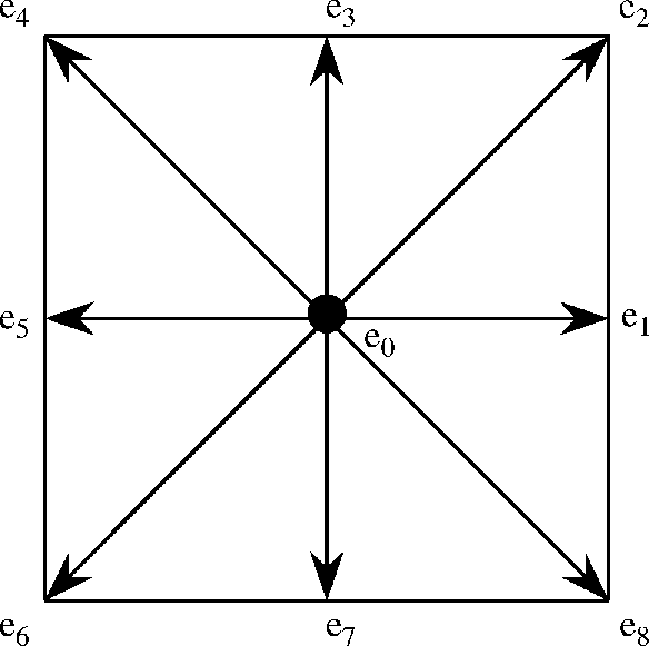
This project aims to use Lattice Boltzmann Method for solving the lid driven flow problem and assess its prediction accuracy and several numerical issues as stated in the problem description. In this project, D2Q9 latice is employed to describe the stream the distribution fuctions along the specified directions. The directions in which 9-bit lattice BGK model evoloves defines following 9 discrete velocities:

\[\begin{split}e_{i} = \left\{\begin{matrix} (0,0) & i=0\;\;\;\;\;\;\;\;\;\; & \\ (\text{cos}[(i-1)\pi/2],\text{sin}[(i-1)\pi/2]) & i=1,2,3,4 & \\ \sqrt{2}(\text{cos}[(i-5)\pi/2 + \pi/4], \text{sin}[(i-5)\pi/2 + \pi/4]) & i=5,6,7,8 & \end{matrix}\right.\end{split}\]

The description of the lattice arrangement and the directions that particle streams are illustrated in the diagram below. Having 9 different velocity vectors, each of the 9 particles (fluid molecules) is moved to neighboring lattices.

Along the defined direction, 9 independent fluid particles are moved and re-located then update their distribution function in time. The evolution equation of the density distribution function is integrated in time as shown below. This step represents the collision process that changes the distribution function for each of 9 particles after streaming. This process will update the fluid macroscopic properties.

\[f_{i}(x_{i}+ce_{i}\Delta t, t+\Delta t) - f_{i}(x_{i}, t) = - \frac{1}{\tau} \left [ f_{i}(x_{i},t) - f_{i}^{\text{eq}}(x_{i},t) \right ]\]

where \(c=\Delta x / \Delta t\), and \(\Delta x\) and \(\Delta t\) are the lattice spacing and the time step, respectively. Here, \(\tau\) is the dimensionless relaxation time that approximates the temporal rate at which instantaneous distribution function evolves and transitions to the equilibrium states. Given kinematic viscosity is taken into account for determining the relaxation time which is determined from following equation:

\[\nu = \frac{2\tau - 1}{6} \Delta x\]

And the \(f_{i}^{\text{eq}}\) expresses the equilibrium density function, which is determined by:

\[f_{i}^{\text{eq}}(x_{i},t) = \omega_{i}\rho + \rho s_{i}(u_{i}(x_{i},t))\]

where

\[s_{i} (u_{i}) = \omega_{i} \left [ e\frac{(e_{i}u_{i})}{c} + 4.5 \frac{(e_{i}u_{i})^{2}}{c^{2}} - 1.5 \frac{u_{i}u_{i}}{c^{2}}\right ]\]

with the weight coefficient:

\[\begin{split}\omega_{i} = \left\{\begin{matrix} \frac{4}{9} & i = 0\;\;\;\;\;\;\;\;\;\; \\ \frac{1}{9} & i = 1,2,3,4 \\ \frac{1}{36} & i = 5,6,7,8 \end{matrix}\right.\end{split}\]

After updating the distribution function, we are then to find fluid density and velocity from the integrated distribution function by assuming the relationship between the distribution function and macroscopic fluid properties:

\[\rho = \sum_{i} f_{i}\]

\[\rho u= \sum_{i} ce_{i}f_{i}\]

Boundary conditions

Treating boundary conditions for Lattice Boltzmann Method is very different from the way with other typical CFD simulation’s approach that directly states flow properties at the boundary. Since the LBM plays with distribution function and derives the macroscopic flow properties from it, the boundary condition should also be treated with specific manipulation of distribution at the boundary lattices.

The issue that arise with the LBM is that there is no further lattices out of the computational domain that accomodate the streamed particles. To cope with this problem, a mid grid bounce-back boundary condition is used to replace the normal 9 direction streaming. On the edge lattices, we assume there is an imaginary lattices right next to the boundary, and when the particles move towards these lattices, it will be bounce back to their original lattice with inversed direction.

For the specific boundary condition of our moving lid on the upper wall, an equation of Zou-He velocity boundary conditions are employed and the specific treatment on this lattice can be made by manipulating the distribution functions as:

\[f_{2} + f_{5} + f_{6} = \rho - \left ( f_{4} + f_{7} + f_{8} + f_{0} + f_{1} + f_{3} \right )\]\[f_{5}-f_{6} = \rho u - \left ( f_{1} + f_{8} - f_{3} - f_{7} \right )\]\[f_{2}+f_{5}+f_{6}=\rho v + \left ( f_{4}+f_{7}+f_{8} \right )\]\[\rho = \frac{1}{1-v}\left ( (f_{0}+f_{1}+f_{3}) -2 (f_{4}+f_{7}+f_{8}) \right )\]